Introduction

For over a century scientists like Sir J.J. Thomson, Ernest Rutherford, and Niels Bohr have studied atomic structure, studies which concluded with the existence of several different models, each attempting to mimic the structure of the atom. In particular, one that is fairly easy to visualize is the Bohr model of the hydrogen atom. This material is covered in depth, along with a complete description of how to calculate energy and wavelengths, in Chapter 7 of your textbook.

The Hydrogen Atom

The structure of the hydrogen atom is very simple: one proton and one electron, a phenomenon known for some time before Bohr . It was also known that the electron was negatively charged while the proton is positively charged. This created some intellectual difficulty to scientists as they did not understand why the electron wouldn’t spiral into the proton—since negative charges are attracted to positive charges—completely destroying the atom. But, since hydrogen was a stable atom, this attraction was obviously not the only rule that governed the behavior of the atom.

The Hydrogen Atom

Understanding why atoms were stable was a very important problem. Even the most advanced physics of the time, Maxwell’s Theory of Electromagnetism, predicted the instability of atoms. There was clearly a very fundamental flaw in their understanding of the universe.

Max Planck, Niels Bohr, and Energy

Prior to Niels Bohr producing his model of the hydrogen atom, Max Planck had postulated that light was composed of photons that carried quanta, a discrete packet of energy. Utilizing this notion, Bohr theorized that since there were well defined states in which atoms could exist, that photons, with just the right energy, could cause transitions between these states. In fact, the reason that the electron did not spiral into the proton was that the atom was actually in one of these stable states. Therefore, Bohr's theory also stated that the electrons were quantized in energy levels.

Quantization

The quantization is often difficult to accept. In the macroscopic world, things are continuous; they can take on any value. For example, a car can travel 17-mph, 18-mph, or 17.5-mph; it is not restricted to only integer values. Things are perceived on such a large scale, that we cannot tell they are quantized, thus appearing as continuous. However, when examined more closely, this continuity no longer holds. In other words, the speed of the car is in fact quantized, but since the difference between two adjacent levels is so small, quantization cannot be observed.

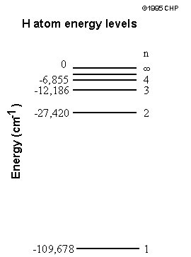
What quantization actually means is that only specific values are allowed. For example, consider a set of steps and a ramp. Since potential energy is a function of height, the potential energy is quantized for the steps, things can exist only on one step or another, they cannot be between steps for a considerable amount of time. Thus, the potential energy increases only in increments of the height of the step. On the other hand, the ramp is not bound by such restrictions. For the ramp, the potential energy is continuous. Overall, it was Bohr's model that made certain predictions about measurable quantities inside atoms, predictions we will be testing in this experiment.

The Predictions and Mathematics

In order to fully understand Bohr's predictions, some math is involved. Bohr's model predicted that the energy of a hydrogen atom was quantized, and that the energy of the atom was dependent on the principle quantum number (n) , which is always an integer. The exact dependence of the energy on this value is complicated to derive, but it turns out that the energy, often abbreviated E_n, is given by the equation shown below where β is a constant based on Planck’s constant, the mass of the electron, and the charge of the electron and given to be ~2.18 x 10^-18 Joules.

From the equation above, we can see that the energy is negative. In technical terms, this means that this energy is a bound state. In its entirety, E_ncan be thought of as a measure of the energy of attraction between the electron and the proton. The smaller the value of n, the closer the electron is to the proton and as a result, the larger the attraction. As n becomes larger, the electron is further away, and the attraction decreases. Overall, as n increases,E_nbecomes less negative, and when n is very large, the fraction is essentially zero, and there is no attraction between the electron and proton. Therefore, the electron is free to go wherever it wants—it is no longer bound to the proton.

It should also be noted that the smallest value of n is one, thus the lowest energy state for hydrogen atoms is the value of β, not zero as one might expect. In fact, the only time the energy of the electron is zero is when it approaches an infinite distance from the nucleus.

Rydberg Equation

By itself, the equation given above is not very useful. There is no energy parameter used to measure the absolute energy, only energy differences can be measured as will now be shown. Consider two possible states of the hydrogen atom that has quantum numbers n_I and n_F. If we consider a transition from the n_I level to the n_F level, the change in energy (ΔE_Level) will be:

The change in energy values from this equation is positive if absorption is occurring and negative when calculating the energy released during an emission.

If the energy difference between these two states is a photon, we expect it to have the energy equal to that calculated. In further detail, the energy of a photon with a frequency v is simply the value of that frequency multiplied by Planck’s constant (h), which is given to be 6.626 x 10^-34 J-sec.

Furthermore, since the frequency is equal to the speed of light (c), 3.00 x 10⁸ m/sec, divided by the wavelength (λ) of the photon in meters:

we can solve for the specific wavelength of light that is associated with a given transition. Specifically, this is known as the Rydberg equation and is shown below.

In this equation, R is known as the Rydberg Constant (1.10 x 10^-2 nm^-1) and takes into account Planck’s constant, as well as the speed of light, and has units that are more practical for calculating wavelengths.

Although mathematically this equation will result in both negative and positive wavelengths, we seldom think of wavelengths as negative values. For example, if nI is smaller than nF, then the wavelength will be positive which corresponds to absorption. If nF is smaller than nI, then the wavelength will be negative which corresponds to an emission. Since the positive and negative conditions are ‘understood’, we simply report both emission and absorption wavelengths as positive values.

Emission and Absorption Series for the Hydrogen Atom

Today’s Adventure

Overall, the Rydberg equation now predicts a measurable value, the wavelengths of light emitted by a transition between two states.  For today’s experiment, n_F will always be 2, the value corresponding to the visible spectrum. Therefore, by substituting values for n_I, corresponding to the visible spectrum of hydrogen, we can predict the wavelengths we should observe.

In this experiment, we will be exciting the hydrogen atom by placing it in an electrical potential. We will also be exciting a variety of cations by heating. Each of these atoms, and ion light sources, will be given as unknowns, it will be your job to use your knowledge of their known wavelengths to identify them.

The Spectroscope

The spectroscope used in today’s experiment has a diffraction grating as its central component. In Figure 7.7 on page 306 of your textbook, there is a picture of a prism and the effect it has on a beam of light. A diffraction grating does basically the same thing, it ‘bends’ light. In particular, the angle at which the light is ‘bent’ depends upon the wavelength of light entering the grating.

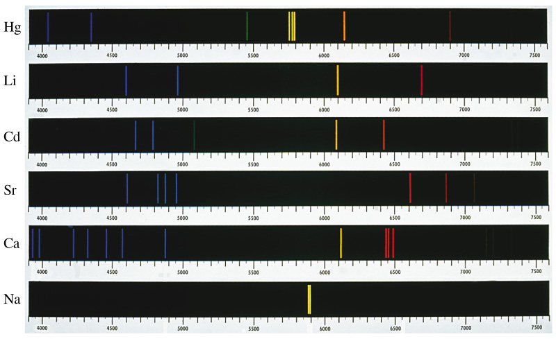
Before we can start accurately measuring the unknown spectrums, we must first calibrate the spectroscope. You will use the known spectrum of helium, given in the table below, to calibrate your spectroscope. Once we plot the measured values of the helium lines against the known values, we can use that graph to determine the actual wavelengths of the unknown lamps and flames provided. Figure 7.9 in Kotz shows several examples of line spectra such as the ones you will be seeing today.